Is Distinct Aggregation Still Considered Harmful?

Back in 2008, Marc Friedman of the SQL Server Query Processor Team wrote a blog entry entitled “Distinct Aggregation Considered Harmful”.

Marc shows a way to work around the poor performance that often results simply from adding the keyword DISTINCT to an otherwise perfectly reasonable aggregate function in a query.

This post is an update to that work, presenting a query optimizer enhancement in SQL Server 2012 that reduces the need to perform the suggested rewrite manually.

First, though, it makes sense for me to cover some broader aggregation topics in general.

Query Plan Options for DISTINCT

There are two main strategies to extract distinct values from a stream of rows.

1. Keep track of the unique values using a hash table.
2. Sort the incoming rows into groups. Return one value from each group.

SQL Server uses the Hash Match operator to implement the hash table option, and Stream Aggregate or Sort Distinct for the sorting option.

Hash Match Aggregate

The optimizer tends to prefer Hash Match Aggregate with:

• Larger number of input rows
• Fewer estimated output groups
• No reason to produce sorted output
• Rows not already sorted on the DISTINCT expression(s).

Larger inputs: Favour hash matching because the algorithm generally scales well (although it does require a memory grant) and can make good use of parallelism.

Fewer groups Better for hashing because it means fewer entries in the hash table. The memory needed to store unique values is proportional to the number of groups (and the size of the group).

Sorting: Hash matching does not require or preserve the order of the incoming row stream.

Example

The AdventureWorks query and plan below show a Hash Match Aggregate building a hash table on values in the Quantity column:

SELECT DISTINCT 
    TH.Quantity
FROM Production.TransactionHistory AS TH
OPTION
(
    RECOMPILE, 
    QUERYTRACEON 9481
);

[

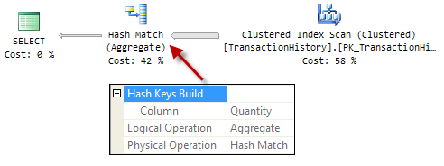
The standard Hash Match Aggregate is a blocking operator. It produces no output until it has processed its entire input stream.

If we restrict the number of rows using TOP or SET ROWCOUNT, the aggregate can operate in a streaming fashion, producing new unique values as soon as they are encountered.

This streaming mode is known as Flow Distinct. It is activated depending on the estimated number of unique values in the stream.

In the example above, the estimated number of output rows from the Hash Match Aggregate is 455 (from statistics). Limiting the query to 455 or fewer rows using TOP or ROWCOUNT produces a Hash Match Aggregate running in Flow Distinct mode:

SET ROWCOUNT 10;

SELECT DISTINCT 
    TH.Quantity
FROM Production.TransactionHistory AS TH
OPTION
(
    RECOMPILE, 
    QUERYTRACEON 9481
);

SET ROWCOUNT 0;

Note the above is a post-execution execution plan because SET ROWCOUNT only takes effect when executed.

This plan is interesting because it limits the output to 10 rows without including a specific TOP operator for that purpose.

TOPis generally preferred to ROWCOUNT for the reasons set out in the documentation for TOP (Transact-SQL). Ignore the part in the Best Practices section that says:

Because SET ROWCOUNT is used outside a statement that executes a query, its value cannot be considered in a query plan.

We have just seen how it can affect a query plan.

For completeness, this is the equivalent TOP query:

SELECT DISTINCT TOP (10)
    TH.Quantity
FROM Production.TransactionHistory AS TH
OPTION
(
    RECOMPILE, 
    QUERYTRACEON 9481
);

The execution plan is:

Stream Aggregate

Performing a DISTINCT is logically the same as applying a GROUP BY on every expression in the SELECT list.

A stream of rows sorted on those GROUP BY expressions has the useful property that all rows with the same GROUP BY values are guaranteed to appear together.

All we need to do is output a single row of GROUP BY keys each time a change in those keys occurs (and at the end of the input stream).

If the required order can be obtained without an explicit Sort operator, the execution plan can use a Stream Aggregate directly:

SELECT DISTINCT 
    TH.ProductID 
FROM Production.TransactionHistory AS TH
OPTION
(
    RECOMPILE, 
    QUERYTRACEON 9481
);

This plan shows an ordered scan of an index on the ProductID column, followed by a Stream Aggregate with a GROUP BY on the same column.

The Stream Aggregate emits a new row each time a new group is encountered, similar to the Hash Match Aggregate running in Flow Distinct mode.

Stream Aggregate does not require a memory grant because it only needs to keep track of one set of GROUP BY expression values at a time.

Sort Distinct

The third alternative is to perform an explicit Sort followed by a Stream Aggregate. The optimizer can often collapse this combination into a single Sort operating in Sort Distinct mode:

SELECT DISTINCT
    P.Color
FROM Production.Product AS P
OPTION
(
    RECOMPILE, 
    QUERYTRACEON 9481
);

To see the original Sort and Stream Aggregate combination, we can temporarily disable the GbAggToSort optimizer rule that performs this transformation:

DBCC RULEOFF('GbAggToSort')

SELECT DISTINCT
    P.Color
FROM Production.Product AS P
OPTION
(
    RECOMPILE, 
    QUERYTRACEON 9481
);

DBCC RULEON('GbAggToSort')

The post-execution plan now shows a regular (non-distinct) Sort followed by the Stream Aggregate:

Distinct Aggregates

The DISTINCT keyword is most commonly used with the COUNT and COUNT_BIG aggregate functions, though it can be specified with a variety of built-in and SQL CLR aggregates.

The interesting thing is that SQL Server always processes distinct aggregates by first performing a DISTINCT (using any of the three methods shown previously), then applying the aggregate (e.g. COUNT) as a second step:

SELECT 
    COUNT_BIG(DISTINCT P.Color) 
FROM Production.Product AS P
OPTION
(
    RECOMPILE, 
    QUERYTRACEON 9481
);

One thing worth highlighting is that COUNT DISTINCT does not count NULLs. The previous query that listed the distinct colours from the Product table produced 10 rows (9 colours and one NULL). The COUNT DISTINCT query returns the value 9.

The execution plan just above uses a Distinct Sort to perform the DISTINCT (which includes the NULL group) and then counts the groups using a Stream Aggregate.

The aggregate expression uses COUNT(expression) rather than COUNT(*) because this correctly eliminates the NULL group produced by the Distinct Sort.

This second example shows a Hash Match Aggregate performing the DISTINCT, followed by a Stream Aggregate to count the non-NULL groups:

SELECT
    COUNT_BIG(DISTINCT TH.Quantity)
FROM Production.TransactionHistory AS TH
OPTION
(
    RECOMPILE, 
    QUERYTRACEON 9481
);

So far, the counting step has always been performed by a Stream Aggregate. This is because it has so far always been a scalar aggregate — an aggregate without a GROUP BY clause.

SQL Server always implements row-mode scalar aggregates using Stream Aggregate. There would be little point using hashing since there will only be one group by definition. Modern versions of SQL Server may use Hash Aggregate for scalar aggregation to take advantage of batch mode processing.

If we add a GROUP BY clause, the final COUNT is no longer a single (scalar) result, so we can get a plan with two Hash Match Aggregates:

SELECT
    TH.ProductID,
    COUNT_BIG(DISTINCT TH.Quantity)
FROM Production.TransactionHistory AS TH
GROUP BY
    TH.ProductID
OPTION
(
    RECOMPILE, 
    QUERYTRACEON 9481
);

In this plan, the rightmost aggregate is performing the DISTINCT, and the leftmost one implements the COUNT with GROUP BY.

Combining Aggregates

The decision to always implement distinct aggregates as separate DISTINCT and aggregate steps makes life easier for the optimizer.

Separating the two operations makes it easier to plan and cost parallelism, partial aggregation, combining similar aggregates, moving aggregates around (for example pushing an aggregate below a join) and so on.

On the downside, it creates problems for queries that include multiple distinct aggregates, or combine a single distinct aggregate with an ‘ordinary’ aggregate.

Multiple Aggregates

There is no problem combining multiple ordinary aggregations into a single operator:

SELECT
    COUNT_BIG(*),
    MAX(TH.ActualCost),
    STDEV(TH.Quantity)
FROM Production.TransactionHistory AS TH
GROUP BY
    TH.TransactionType
OPTION
(
    RECOMPILE, 
    QUERYTRACEON 9481
);

The single Hash Match Aggregate operator concurrently computes the COUNT_BIG, MAX, and STDEV aggregates on the incoming stream.

Multiple Distinct Aggregates

This next query does a similar thing, but with three DISTINCT aggregations on the stream:

SELECT 
    COUNT_BIG(DISTINCT TH.ProductID), 
    COUNT_BIG(DISTINCT TH.TransactionDate), 
    COUNT_BIG(DISTINCT TH.Quantity)
FROM Production.TransactionHistory AS TH
OPTION
(
    RECOMPILE, 
    QUERYTRACEON 9481
);

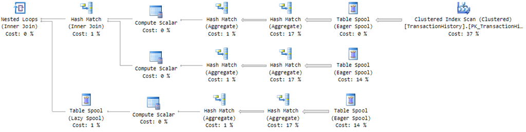
It produces a more complex query plan:

The issue here is that once a DISTINCT has been performed on a stream, the stream no longer contains the columns necessary to perform the other DISTINCT operations.

To work around this, the optimizer builds a plan that reads the source stream once per DISTINCT, computes the aggregates separately, and then combines the results using a cross join (which is safe because these are all scalar aggregates, guaranteed to produce exactly one row each).

The same basic pattern is employed if the query contains an outer GROUP BY clause, but instead of cross joins there will be inner joins on the GROUP BY columns.

More often than not, the source of rows will not be an unrestricted table scan. Where the source is complex (and therefore expensive to re-run for each distinct aggregate) or where a filter significantly reduces the number of rows, the query optimizer may choose to Eager Spool the source rows and replay them once per distinct aggregate:

SELECT 
    COUNT_BIG(DISTINCT TH.ProductID), 
    COUNT_BIG(DISTINCT TH.TransactionDate), 
    COUNT_BIG(DISTINCT TH.Quantity)
FROM Production.TransactionHistory AS TH
WHERE
    TH.ActualCost < $5
GROUP BY
    TH.TransactionType
OPTION
(
    RECOMPILE, 
    QUERYTRACEON 9481
);

This is a plan shape that you are likely to encounter in the real world, since most queries will likely have a filtering condition or have a row source that is more complex than a simple scan of an index or table.

For queries over larger tables than the AdventureWorks database provides, this plan is likely to perform poorly.

Aside from the obvious concerns, inserting rows into a spool has to be performed on a single thread (like most data modification operations).

Another limitation is that this spool does not support parallel scan for reading, so the optimizer is very unlikely to restart parallelism after the spool (or any of its replay streams).

In queries that operate on large data sets, the parallelism implications of the spool plan can be the most important cause of poor performance.

Performing Multiple Distinct Aggregates Concurrently

If SQL Server were able to perform the whole COUNT DISTINCT aggregate in a single operator (instead of splitting the DISTINCT and COUNT into two steps), there would be no reason to split plans with spools as seen above.

This could not be done with a Stream Aggregate because that operator requires the stream to be sorted on the DISTINCT expression, and it is not possible to sort a single stream in more than one way at the same time.

On the other hand, the Hash Match Aggregate does not require sorted input — it keeps the distinct values in a hash table, remember. So, it ought to be possible to design a Hash Match Aggregate that computes COUNT DISTINCT in a single operation.

We can test this idea with a User-Defined Aggregate (UDA) – SQL Server 2008 or later required:

using System;
using System.Collections.Generic;
using System.Data.SqlTypes;
using System.IO;
using Microsoft.SqlServer.Server;

[SqlUserDefinedAggregate
    (
    Format.UserDefined,
    IsInvariantToDuplicates = true,
    IsInvariantToNulls = true,
    IsInvariantToOrder = true,
    IsNullIfEmpty = false,
    MaxByteSize = -1
    )
]

public struct CountDistinctInt : IBinarySerialize
{
    // The hash table
    private Dictionary<int, object> dict;

    // Recreate the hash table for each new group
    public void Init()
    {
        dict = new Dictionary<int, object>();
    }

    // Ignore NULLs, store key values in the hash table
    public void Accumulate(SqlInt32 Data)
    {
        if (!Data.IsNull)
        {
            dict[Data.Value] = null;
        }
    }

    // Merge partial aggregates
    public void Merge(CountDistinctInt Group)
    {
        foreach (var item in Group.dict.Keys)
        {
            dict[item] = null;
        }
    }

    // Return the DISTINCT COUNT result
    public int Terminate()
    {
        return dict.Count;
    }

    // Required by SQL Server to serialize this object
    void IBinarySerialize.Write(BinaryWriter w)
    {
        w.Write(dict.Count);
        foreach (var item in dict.Keys)
        {
            w.Write(item);
        }
    }

    // Required by SQL Server to deserialize this object
    void IBinarySerialize.Read(BinaryReader r)
    {
        var recordCount = r.ReadInt32();

        dict = new Dictionary<int, object>(recordCount);

        for (var i = 0; i < recordCount; i++)
        {
            dict[r.ReadInt32()] = null;
        }
    }
}

This UDA does nothing more than create a hash table, add (non-NULL) values to it, and return the count of values when aggregation is complete. The hash table automatically takes care of duplicates.

There is a little extra infrastructure code in there to allow SQL Server to serialize and deserialize the hash table when needed, and merge partial aggregates, but the core of the function is just four lines of code. The example above only aggregates integer values, but it is easy to extend the idea to include other types.

Armed with the integer and datetime versions of the UDA, I now return to the multiple-distinct-count query that caused all the spooling, with COUNT DISTINCT replaced by UDA references:

SELECT 
    dbo.CountDistinctInt(TH.ProductID), 
    dbo.CountDistinctDateTime(TH.TransactionDate), 
    dbo.CountDistinctInt(TH.Quantity)
FROM Production.TransactionHistory AS TH
WHERE
    TH.ActualCost < $5
GROUP BY
    TH.TransactionType
OPTION
(
    RECOMPILE, 
    QUERYTRACEON 9481
);

Instead of all the Eager Spools, we now get this query plan:

You may be surprised to see that the three distinct count aggregates are being performed by a Stream Aggregate — after all, I just finished explaining why a Stream Aggregate could not possibly do what we want here.

The thing is that all CLR UDAs are interfaced to query plans using the Stream Aggregate model. The fact that this UDA uses a hash table internally does not change that external implementation fact.

The Sort in this plan is there to ensure that groups of rows arrive at the Stream Aggregate interface in the required GROUP BY order. This is so SQL Server knows when to call the Init() and Terminate() methods on our UDA.

The COUNT DISTINCT aggregation that is happening inside the UDA for each group could not care less about ordering, of course. (In case you were wondering, yes, the UDA produces the same results as the original T-SQL code).

The point here is to demonstrate that multiple DISTINCT COUNT operations can be performed within a single operator, not that UDAs are necessarily a great way to do that in general.

As far as performance is concerned, the original spool query runs for around 220ms. The UDA settles down around 160ms, which isn’t bad, all things considered.

We can improve the performance of the T-SQL query by rewriting it to avoid the spools by scanning the source table three times (this executes in around 75ms).

Part of the problem here (to go with the spool plan issues mentioned earlier) is that the optimizer assumes that all queries start executing with an empty data cache. It also does not account for the fact that the three scans complete sequentially, so the pages are extremely likely to be available from memory for the second and third scans.

The rewrite and resulting execution plan are below:

WITH 
    Stream AS 
    (
        SELECT 
            TH.TransactionType, 
            TH.ProductID, 
            TH.TransactionDate, 
            TH.Quantity 
        FROM Production.TransactionHistory AS TH
        WHERE 
            TH.ActualCost < $5
    ),
    CountDistinctProduct AS
    (
    SELECT 
        TransactionType, 
        COUNT_BIG(DISTINCT ProductID) AS C
    FROM Stream 
    GROUP BY 
        TransactionType
    ),
    CountDistinctTransactionDate AS
    (
    SELECT 
        TransactionType, 
        COUNT_BIG(DISTINCT TransactionDate) AS C
    FROM Stream 
    GROUP BY 
        TransactionType
    ),
    CountDistinctQuantity AS
    (
    SELECT 
        TransactionType, 
        COUNT_BIG(DISTINCT Quantity) AS C
    FROM Stream 
    GROUP BY 
        TransactionType
    )
SELECT
    P.c,
    D.c,
    Q.c
FROM CountDistinctProduct AS P
JOIN CountDistinctTransactionDate AS D
    ON D.TransactionType = P.TransactionType
JOIN CountDistinctQuantity AS Q
    ON Q.TransactionType = D.TransactionType
OPTION
(
    RECOMPILE, 
    QUERYTRACEON 9481
);

Combining a Single Distinct Aggregate with other Aggregates

Marc Friedman’s blog post presented a way to rewrite T-SQL queries that contain a single distinct aggregate and one or more non-distinct aggregates so as to avoid spools or reading the source of the rows more than once.

The essence of the method is to aggregate first by the GROUP BY expressions in the query and the DISTINCT expressions in the aggregate, and then to apply some relational math to aggregate those partial aggregates to produce the final result.

I encourage you to read the full post to see all the detail, but I will quickly work through an example here too. Note that these queries use the AdventureWorksDW database.

SELECT
    DP.EnglishProductName,
    SUM(FRS.SalesAmount),
    COUNT_BIG(DISTINCT FRS.SalesTerritoryKey)
FROM dbo.FactResellerSales AS FRS
JOIN.dbo.DimProduct AS DP
    ON FRS.ProductKey = DP.ProductKey
GROUP BY
    DP.EnglishProductName
OPTION
(
    RECOMPILE, 
    MAXDOP 1,
    QUERYTRACEON 9481
);

This query contains a regular SUM aggregate and a COUNT DISTINCT. As expected, the query optimizer produces a plan with an Eager Spool:

To the left of the spool, the top branch performs the DISTINCT followed by the COUNT per group. The replay on the lower branch of the plan computes the SUM per group. The two branches join on the common GROUP BY column, EnglishProductName.

The rewrite starts by grouping on EnglishProductName (the GROUP BY expression) and SalesTerritoryKey (the DISTINCT expression) to produce a partial aggregate:

SELECT 
    DP.EnglishProductName, 
    FRS.SalesTerritoryKey, 
    SUM(FRS.SalesAmount) AS ssa
FROM dbo.DimProduct AS DP
JOIN dbo.FactResellerSales AS FRS
    ON FRS.ProductKey = DP.ProductKey
GROUP BY 
    FRS.SalesTerritoryKey, 
    DP.EnglishProductName
OPTION
(
    RECOMPILE, 
    MAXDOP 1,
    QUERYTRACEON 9481
);

This query contains no distinct aggregates, so we get a plan with an ordinary join and an ordinary SUM aggregate:

To produce the results specified by the original query, we now need to SUM the partial SalesAmount sums, and COUNT (ignoring NULLs) the SalesTerritoryKeyvalues.

The final rewrite looks like this:

WITH PartialAggregate AS
(
    SELECT 
        DP.EnglishProductName, 
        FRS.SalesTerritoryKey, 
        SUM(FRS.SalesAmount) AS SSA
    FROM dbo.DimProduct AS DP
    JOIN dbo.FactResellerSales AS FRS 
        ON FRS.ProductKey = DP.ProductKey
    GROUP BY 
        FRS.SalesTerritoryKey, 
        DP.EnglishProductName
)
SELECT
    PA.EnglishProductName, 
    SUM(PA.SSA),
    COUNT_BIG(PA.SalesTerritoryKey)
FROM PartialAggregate AS PA
GROUP BY PA.EnglishProductName
OPTION
(
    RECOMPILE, 
    MAXDOP 1,
    QUERYTRACEON 9481
);

The execution plan adds another layer of aggregation on top of the partial aggregate plan from the previous step:

This plan avoids the Eager Spools seen earlier and improves execution time from 320ms to 95ms.

On larger sets, where parallelism becomes important and the spools might need to use physical tempdb storage, the potential gains are correspondingly larger.

New in SQL Server 2012

The good news is that SQL Server 2012 adds a new optimizer rule ReduceForDistinctAggs to perform this rewrite automatically on the original form of the query.

This is particularly good because the rewrite, while ingenious, can be somewhat inconvenient to do in practice, and all too easy to get wrong (particularly ensuring that NULL partially-aggregated groups are handled correctly).

With the new optimizer rule, this query:

SELECT
    DP.EnglishProductName,
    SUM(FRS.SalesAmount),
    COUNT_BIG(DISTINCT FRS.SalesTerritoryKey)
FROM dbo.FactResellerSales AS FRS
JOIN.dbo.DimProduct AS DP 
    ON FRS.ProductKey = DP.ProductKey
GROUP BY
    DP.EnglishProductName
OPTION
(
    RECOMPILE, 
    MAXDOP 1,
    QUERYTRACEON 9481
);

…can directly produce this execution plan:

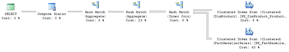
This transformation is only valid for queries with a single distinct aggregate (and at least one non-distinct aggregate of course).

If your query contains multiple distinct aggregates, it may not help you directly, though you may be able to refactor the T-SQL to take advantage.

If you want to see SQL Server 2012 or later produce the Eager Spool plan instead (created by the long-standing ExpandDistinctGbAgg rule), you can disable the new rule with:

DBCC RULEOFF ('ReduceForDistinctAggs')

…and then recompile. Don’t forget to enable it again afterward using DBCC RULEON or by reconnecting to the server. As always, this information is for educational purposes only and is not suitable for production use.

Even with the new rule enabled, you may still see the spool or multiple-scan plan from time to time. As always, the optimizer explores many alternative plan fragments, and chooses the combination that looks cheapest overall.

In some cases, the optimizer may still choose the spool plan, though it probably won’t be the right decision in practice.

Thanks for reading. Please consider voting for the feedback suggestion Allow OPTION(HASH GROUP) with SQLCLR UDAs.

© Paul White
email: SQLkiwi@gmail.com
twitter: @SQL_Kiwi