Optimizing T-SQL queries that change data

Most tuning efforts for data-changing operations concentrate on the SELECT side of the query plan. Sometimes people will also look at storage engine considerations (like locking or transaction log throughput) that can have dramatic effects. A number of common practices have emerged, such as avoiding large numbers of row locks and lock escalation, splitting large changes into smaller batches of a few thousand rows, and combining a number of small changes into a single transaction in order to optimize log flushes.

This is all good, but what about the data-changing side of the query plan — the INSERT, UPDATE, DELETE, or MERGE operation itself — are there any query processor considerations we should take into account? The short answer is yes.

The query optimizer considers different plan options for the write-side of an execution plan, though there isn’t a huge amount of T-SQL language support that allows us to affect these choices directly. Nevertheless, there are things to be aware of, and things we can look to change.

Side note:

In this post I am going to use the term update (lower case) to apply to any operation that changes the state of the database (INSERT, UPDATE, DELETE, and MERGE in T-SQL). This is a common practice in the literature, and is used inside SQL Server too as we will see.

The Three Basic Update Forms

Query plans execute using a demand-driven iterator model, and updates are no exception. Parent operators drive child operators (to the right of the parent) to do work by asking them for a row at a time.

Take the following AdventureWorks INSERT for example:

DECLARE @T table (ProductID integer NOT NULL);

INSERT @T (ProductID) 
SELECT P.ProductID 
FROM Production.Product AS P;

Plan execution starts at the far left, where you can think of the green T-SQL INSERT icon as representing rows returned to the client. This root node asks its immediate child operator (the Table Insert) for a row. The Table Insert requests a row from the Index Scan, which provides one. This row is inserted into the heap, and an empty row is returned to the root node (if the INSERT query contained an OUTPUT clause, the returned row would contain data).

This row-by-row process continues until all source rows have been processed. Notice that the XML showplan output shows the Heap Table Insert is performed by an Update operator internally.

1. Wide, per-index updates

Wide (aka per-index) update plans have a separate update operator for each clustered and nonclustered index.

An example per-index update plan is shown below:

This plan updates the base table using a Clustered Index Delete operator. This operator may also read and output extra column values necessary to find and delete rows from nonclustered indexes.

The iterative clustered index delete activity is driven by the Eager Table Spool on the top branch. The spool is eager because it stores all the rows from its input into a worktable before returning the first row to its parent operator (the Index Delete on the top branch). The effect is that all qualifying base table rows are deleted before any nonclustered index changes occur.

The spool in this plan is a common subexpression spool. It is populated once, then acts as a row source for multiple consumers. In this case, the contents of the spool are consumed first by the top-branch Index Delete, which removes index entries from one of the nonclustered indexes.

When the Sequence operator switches to asking for rows from the lower branch, the spool is rewound and replays its contents to delete rows from the second nonclustered index. Note that the spool contains the union of all columns required for all the nonclustered index changes.

2. Narrow, per-row updates

Narrow (aka per-row) updates have a single update operator that maintains the base table (heap or clustered index), and one or more nonclustered indexes. Each row arriving at the update operator updates all indexes associated with the operator before processing the next row. An example:

DECLARE @T table 
(
    pk integer PRIMARY KEY,
    col1 integer NOT NULL UNIQUE, 
    col2 integer NOT NULL UNIQUE
);

DECLARE @S table 
(
    pk integer PRIMARY KEY, 
    col1 integer NOT NULL,
    col2 integer NOT NULL);

INSERT @T (pk, col1)
SELECT
    S.pk,
    S.col1 
FROM @S AS S;

The execution plan viewed using Sentry One Plan Explorer shows the nonclustered index maintenance explicitly. Hover over the Clustered Index Insert for a tooltip showing the names of the nonclustered indexes involved:

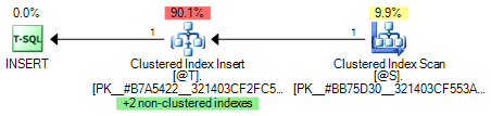
In SQL Server Management Studio, there is no information about the nonclustered index maintenance in the graphical plan or tooltips. We need to click on the update operator (Clustered Index Insert) and then check the Properties window:

The Object subtree shows the clustered index and two nonclustered indexes being maintained.

Cost-based choice

The query optimizer uses cost-based reasoning to decide whether to update each nonclustered index separately (per-index) or as part of the base table changes (per-row).

An example that updates one nonclustered index per-row, and another per-index is shown below:

CREATE TABLE #T 
(
    pk integer IDENTITY PRIMARY KEY,
    col1 integer NOT NULL,
    col2 varchar(8000) NOT NULL DEFAULT ''
);

CREATE INDEX nc1 ON #T (col1);
CREATE INDEX nc2 ON #T (col1) INCLUDE (col2);

INSERT #T
    (col1)
SELECT
    N.n
FROM dbo.Numbers AS N
WHERE
    N.n BETWEEN 1 AND 251;

The combination strategy can be seen with Plan Explorer:

The details are also displayed in the SSMS Properties window when the Clustered Index Insert operator is selected.

3. Single-operator updates

The third form of update is an optimization of the per-row update plan for very simple operations. The cost-based optimizer still emits a per-row update plan, but a rewrite is subsequently applied to collapse the reading and writing operations into a single operator:

DECLARE @T AS TABLE 
(
    pk integer PRIMARY KEY, 
    col1 integer NOT NULL
);

-- Simple operations
INSERT @T (pk, col1) VALUES (1, 1000);
UPDATE @T SET col1 = 1234 WHERE pk = 1;
DELETE @T WHERE pk = 1;

The complete execution plans (and extracts from the XML plans) are shown below:

The UPDATE and DELETE plans have been collapsed to a Simple Update operation, while the INSERT is simplified to a Scalar Insert.

We can see the optimizer output tree with trace flag 8607:

DECLARE @T table
(
    pk integer PRIMARY KEY, 
    col1 integer NOT NULL
);

DBCC TRACEON (3604, 8607);

INSERT @T (pk, col1) VALUES (1, 1000) OPTION (RECOMPILE);
UPDATE @T SET col1 = 1234 WHERE pk = 1 OPTION (RECOMPILE);
DELETE @T WHERE pk = 1 OPTION (RECOMPILE);

DBCC TRACEOFF (3604, 8607);

The message window output for the INSERT statement shown above is:

*** Output Tree: (trivial plan) ***
PhyOp_StreamUpdate
    (INS TBL: @T, iid 0x1 as TBLInsLocator(QCOL: .pk ) REPORT-COUNT), {
        - QCOL: .pk= COL: Expr1002 
        - QCOL: .col1= COL: Expr1003 } 
    PhyOp_ConstTableScan (1) COL: Expr1002  COL: Expr1003 
        ScaOp_Const TI(int,ML=4) XVAR(int,Not Owned,Value=1)
        ScaOp_Const TI(int,ML=4) XVAR(int,Not Owned,Value=1000)

Notice the two physical operators: A Constant Scan (in-memory table) containing the literal values specified in the query; and a Stream Update that performs the database changes per row.

All three statements produce a similar optimizer tree output (and all use a stream update). We can prevent the single-operator optimization being applied with undocumented trace flag 8758:

DECLARE @T table
(
    pk integer PRIMARY KEY, 
    col1 integer NOT NULL
);

DBCC TRACEON (8758);

INSERT @T (pk, col1) VALUES (1, 1000) OPTION (RECOMPILE);
UPDATE @T SET col1 = 1234 WHERE pk = 1 OPTION (RECOMPILE);
DELETE @T WHERE pk = 1 OPTION (RECOMPILE);

DBCC TRACEOFF (8758);

This exposes the expanded per-row update plans produced by the optimizer before the single-operator rewrite:

Single operator plans can be significantly more efficient than the multiple-operator form in the right circumstances, for example if the plan is executed very frequently.

Update plan optimizations

From this point forward, I’m going to use AdventureWorks DELETE examples, but the general points apply equally well to INSERT, UPDATE, and MERGE as well.

The examples will not have a complicated SELECT component, because I want to concentrate on the update side of the plan rather than the reading side.

Per-row updates

It’s worth emphasising that narrow update plans are an optimization that is not available for every update query (except for Hekaton where they are the default).

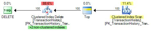
The optimizer favours a per-row plan if the expected number of rows at the update operator is low. In the example below, the optimizer expects to delete 25 rows:

This plan updates the base table (a clustered index in this case) and all nonclustered indexes in sequence per row. The row source here is an ordered scan of a nonclustered index, which means rows will not generally be presented in clustered index key order to the update operator.

An unordered stream like this tends to result in random I/O (assuming physical I/O is required). If the plan is expected to process only a small number of rows, the optimizer decides it is not worth adding extra operations to encourage a sequential I/O access pattern.

Unordered Prefetch

If the expected number of rows is a bit larger, the optimizer may decide to build a plan that applies prefetching to one or more update operators.

The basic idea is the same as ordinary prefetching (a.k.a read-ahead) for scans and range seeks. The engine looks ahead at the keys of the incoming stream and issues asynchronous I/O for pages that will be needed by the update operator soon.

Prefetching can help reduce the impact of the expected random I/O. An example of prefetching on the update operator is shown below for the same DELETE query with an expected cardinality of 50 rows:

The prefetching is unordered from the perspective of the clustered index. Neither SSMS nor Plan Explorer show the prefetch information prominently.

In Plan Explorer, we need to have the With Unordered Prefetch optional column selected. To do this, switch to the Plan Tree tab, open the Column Chooser, and drag the column to the grid. The unordered prefetch property is ticked for the Clustered Index Delete operator in the screenshot below:

In SSMS, click on the Clustered Index Delete icon in the graphical plan, and then look in the Properties window:

If the query plan were reading from the clustered index (instead of a nonclustered index), the read operation would issue regular read-ahead, so there would be no point prefetching from the Clustered Index Delete as well.

The example below shows the expected cardinality increased to 100, where the optimizer switches from scanning the nonclustered index with unordered prefetching to scanning the clustered index with regular read-ahead. No prefetching occurs on the update operator in this plan:

Where the plan property With Unordered Prefetch is not set, it is simply omitted — it does not appear set to False as you might expect.

Ordered Prefetch

Where rows are expected to arrive at an update operator in non-key order, the optimizer might consider adding an explicit Sort operator. The idea is that presenting rows in key order will encourage sequential I/O for the index pages.

The optimizer weighs the cost of sorting against the expected benefits of avoiding random I/O. The execution plan below shows an example of a sort being added for this reason:

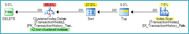
The Sort is on Transaction ID, the clustering key for this table. With the incoming stream now sorted, the update operator can use ordered prefetching.

The plan is still scanning the nonclustered index on the read side, so read-ahead issued by that operator does not bring in the clustered index pages needed by the update operator.

Ordered prefetching tends to result in sequential I/O, compared with the mostly random I/O of unordered prefetching. The With Ordered Prefetch column is also not shown by default by Plan Explorer, so it needs to be added as we did before:

Not every update operator with ordered prefetching requires a Sort. If the optimizer finds a plan that naturally presents keys in nonclustered index order, an update operator may still use ordered prefetching to pull pages we are about to modify into memory before they are requested by the update operator.

DML Request Sort

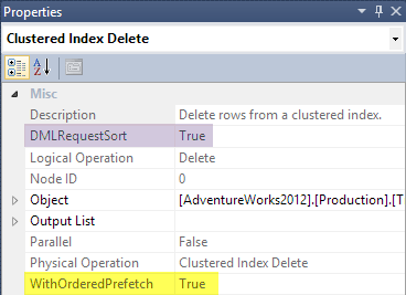
When the optimizer decides to explore a plan alternative that requires ordered input to an update operator, it will set the DML Request Sort property for that operator.

Plan Explorer shows this setting in the update operator tooltip:

SSMS shows With Ordered Prefetch and DML Request Sort in the Properties window:

Nonclustered index updates

Sorting and ordered prefetching may also be considered for the nonclustered indexes in a wide update plan:

This plan shows all three update operators with DML Request Sort set.

The Clustered Index Delete does not require an explicit sort because rows are being read (with internal ordering guarantees) from the Clustered Index Scan.

The two non-clustered indexes do require explicit sorting. Both nonclustered index update operators also use ordered prefetching; the clustered index update does not because the prior scan automatically invokes read-ahead for that index.

The next example shows that each update operator is considered separately for the various optimizations:

That plan features unordered prefetching on the Clustered Index Delete (because the row source is a scan of a nonclustered index), an explicit Sort with ordered prefetching on the top branch Index Delete, and unordered prefetching on the bottom branch Index Delete.

The per-index and per-row update plan

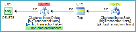
Is the following a per-index or per-row update plan?

It appears to be a per-index plan because there are two separate update operators, but there is no blocking operator (Eager Spool or Sort) between the two.

This plan is a pipeline. Each row returned from the seek will be processed first by the Clustered Index Delete and then by the Index Delete. In that sense, both updates (clustered and nonclustered) are per-row.

Anyway, the important thing is not the terminology, it is being able to interpret the plan. Now we know what the various optimizations are for, we can see why the optimizer chose the plan above over the seemingly equivalent but more efficient-looking narrow plan:

The narrow plan has no prefetching. The Seek provides read-ahead for the clustered index pages, but the single non-clustered index has nothing to prefetch any pages from disk it might need.

By contrast, the wide update plan has two update operators. The Clustered Index Delete has no prefetching for the same reason as in the narrow plan, but the Index Delete has unordered prefetching enabled.

So, although the smaller narrow plan looks like it ought to be more efficient, it might perform less well if nonclustered index pages are required from disk and unordered prefetching proves effective.

On the other hand, if all required nonclustered index pages are in memory at the time the query is executed, the wide plan might perform less well since it features an extra operator and has to perform work associated with prefetching (even though ultimately no physical reads are issued).

Performance Impacts

You may have noticed a lack of performance numbers (I/O statistics, elapsed times and so on) in this post. There is a good reason for this. The optimizations presented here are quite dependent on SQL Server configuration and hardware. I don’t want you drawing general conclusions based on the performance of the rather ordinary single spinning hard drive in my laptop, the 256MB of RAM I have allowed for my SQL Server 2012 instance, and some rather trivial AdventureWorks examples.

Which Optimizations are Good?

If the data structures you are changing are very likely to be in memory, and/or if you have a very fast random I/O system, the optimizer’s goal of minimizing random I/O and enhancing sequential I/O may not make much sense for you. The strategies the optimizer employs may well end up costing more than they save.

On the other hand, if your system has a much smaller buffer pool than database working set size, and your I/O system works very much faster with large sequential I/O than with smaller random I/O requests, you should generally find the optimizer makes reasonable choices for you, subject to the usual caveats about useful up-to-date statistics and accurate cardinality estimations.

If your system fits the optimizer’s model, at least to a first approximation, you will usually find that narrow update plans are best for low row-count update operations, unordered prefetching helps a bit when more rows are involved, ordered prefetching helps more, and explicit sorts before nonclustered index updates help most of all for the largest sets. That is the theory, anyway.

What are the Problems?

The problem I see most often is with the optimization that is supposed to help most: The explicit Sort before a nonclustered index update.

The idea is that sorting the input to the index update in key order promotes sequential I/O, and often it does. The problem occurs if the workspace memory allocated to the Sort proves to be too small to perform it entirely in memory. The memory grant is fixed based on cardinality estimation and row size estimates, and may be reduced if the server is under memory pressure at the time.

A Sort that runs out of memory spills whole sort runs to physical tempdb disk, often repeatedly. This is often not good for performance, and can result in queries that complete very much slower than if the Sort had not been introduced at all.

Note: SQL Server reuses the general Sort operator here — it does not have a Sort specially tuned for updates that could make a best effort to sort within the memory allocated, but never spill to disk.

The narrow plan optimization can cause problems where it is selected due to a low cardinality estimate, where several nonclustered indexes need to be maintained, the necessary pages are not in memory, and the I/O system is slow at random reads.

The ordered and unordered prefetch options cause problems much more rarely. For a system with all data in memory, there is a small but possibly measurable impact due to the prefetch overhead (finding pages to consider read-ahead for, checking to see if they are already in the buffer pool, and so on). Even if no asynchronous I/O is ever issued by the worker, it still spends time on the task that it could spend doing real work.

What options are there?

The usual answer to deal with poor execution plan choices due to a system’s configuration or performance characteristics not matching the optimizer’s model is to try different T-SQL syntax, and/or to try query hints.

There are times when it is possible to rewrite the query to get a plan that performs better, and other times where rethinking the problem a bit can pay dividends. Various creative uses of partitioning, minimal logging, and bulk loading are possible in some cases, for example.

There are very few hints that can help with the update side of a plan that does not respond to the usual tricks, however. The two I use most often affect the optimizer’s cardinality estimation — OPTION (FAST n) and a trick involving TOP and the OPTIMIZE FOR query hint.

OPTION (FAST n) affects cardinality estimates in a plan by setting a final row goal, but its effects can be difficult to predict, and may not have much of an effect if the plan contains blocking operators. Anyway, the general idea is to vary the value of ‘n’ in the hint until the optimizer chooses the desired plan shape or optimization options as described in this post. Best of luck with that.

The idea with TOP is similar, but often tends to work better in my experience. The trick is to declare a bigint variable with the number of rows the query should return (or a very large value such as the maximum value of a bigint if all rows are required), use that as the parameter to a TOP, and then use the OPTIMIZE FOR hint to set a value for ‘n’ that the optimizer should use when considering alternative plans. This option is particularly useful for encouraging a narrow plan.

Most of the examples in this post used the TOP trick in the following general form:

DECLARE @n bigint = 9223372036854775807;

DELETE TOP (@n) 
FROM Production.TransactionHistory
OPTION (OPTIMIZE FOR (@n = 50));

Magic trace flags

There are trace flags that affect the optimizations discussed in this post. They are undocumented and unsupported, and may only work on some versions, but they can be handy to validate a performance analysis, or to generate a plan guide for a particularly crucial query. They can also be fun to play with on a personal system to explore their effects. The main ones that affect the optimizations described here are:

2332 : Force DML Request Sort
8633 : Enable prefetch only
8744 : Disable prefetch only
8758 : Disable rewrite to a single operator plan
8790 : Force a wide update plan
8795 : Disable DML Request Sort
9115 : Disable optimized NLJ and prefetch

These trace flags can all be manipulated using the usual DBCC commands or enabled temporarily for a particular query using the OPTION (QUERYTRACEON xxxx) hint.

Final Thoughts

The optimizer has a wide range of choices when building the writing side of an update plan. It may choose to update one or more indexes separately, or as part of the base table update. It may choose to explicitly sort rows as part of a per-index update strategy, and may elect to perform unordered or ordered prefetching as well.

As usual, these decisions are made based on costs computed using the optimizer’s model. This model may not always produce plans that are optimal for your hardware (and as usual the optimizer’s choices are only as good as the information you give it).

If a particular update query is performance critical for you, make sure cardinality estimates are reasonably accurate. Test with alternate syntax and/or trace flags to see if an alternative plan would perform significantly better in practice. It is usually possible to use documented techniques like TOP clauses and OPTIMIZE FOR hints to produce an execution plan that performs well. Where that is not possible, more advanced tricks and techniques like plan guides may be called for.

Thanks for reading. I hope this post was interesting and provided some new insights into update query optimization.

© Paul White
email: SQLkiwi@gmail.com
twitter: @SQL_Kiwi